Project Portfolio Management: Project Selection

IT outsourcing is a growing industry. It allows industries to focus on their core business while specialized companies manage their IT infrastructure, operations and application development. This strategy has been deployed with success in a large number of organizations around the world allowing both sides of the partnership to grow. IT is thus deployed as a service.

When discussing IT outsourcing, the main distinction is whether infrastructure and / or applications are outsourced. In the remaining part of the article, infrastructure outsourcing will be referred to as IO while application outsourcing will be referred to as AO.

IO focuses on the IT components of the organization: from network backbone (routers, switches, firewall ...) to end-users workstations without forgetting servers (mail, web, ERP, …) or support. In addition of the daily operations of maintenance / upgrade / etc..., IO might as well include the implementation of new projects. AO on the other side takes care of application development and ensures that it supports the business in the daily work of the end-users (whether they are manufacturing employees, clerks, salesperson, etc...).

In the example that we consider, we analyze a case of a production company (Production Inc.) that outsources both infrastructure and application development to an external IT partner (IT Inc.). IT Inc. is therefore responsible for all operations and application development for Production Inc in a full IO and AO deal. In addition, IT Inc. is a key advisor of Production Inc. and, due to its profound knowledge of all IT operations, is in a good position to suggest potential improvements and new projects to implement the required changes. On a yearly basis, IT Inc. gathers inputs from all its employees in order to suggest to Production Inc. the best projects that will support its operations and growth. Furthermore, the executive team of Production Inc. also has a list of projects that they would like to conduct and therefore need to select which projects are worth their investment.

In this context, Production Inc. needs to combine its own projects and the different projects submitted by IT Inc. and will need to evaluate which are the best. This evaluation cannot only be based on the costs (implementation, maintenance, training ...), which makes the selection of projects a complex task. In this particular scenario, Production Inc. has identified a number of criteria that they wish to consider before taking a decision on which projects to implement. Those criteria have been divided in two main categories: price and quality, each category subdivided as shown below:

1. Costs
   1. Project: these criteria reflect the direct costs visible to Production Inc.
      1. Initial Investment: this is the cost of additional components that need to be added to the infrastructure (for instance new servers, new network routers ...). It is expressed in Euros.
      2. Implementation cost: this is the cost of labor necessary to implement the project (installation, configuration, integration ...). It is expressed in Euros.
   2. Operational: this reflects the costs once the project has been completed and that it is fully functional (i.e. put in production)
      1. Daily operations: this is the difference of costs between daily operations before the implementation of the project and once it is completed. If the system is less expensive to work with on a daily basis, this will be a negative value. It is expressed in Euros.
      2. Knowledge transfer: this is the price of transferring the knowledge from the people who realized the project to the people who will maintain the solution in place. It is expressed in Euros.
2. Quality
   1. Logistic: this subcategory reflects the planning of the project in terms of required efforts and length
      1. Length: this is the expected length of the project, from the planning phase until it is deployed into the production environment. It is expressed in days.
      2. Man days: this is the required effort and it highlights how much time the different resources working on the project are going to spend. This is expressed in Man Days (MD) where 1 MD is the time spent by one resource during one day (8h). This criterion is not directly related to the length of the project as it depends on the time repartition.
   2. Strategy: this subcategory assesses how the projects align with the strategy defined by the executive team of Production Inc and which risks are involved with the implementation of the project.
      1. Strategy alignment: this criterion measures how the project is aligned with the predefined strategy of Production Inc against a qualitative scale. The scale is [10%; 20%; 40%; 60%; 80%; 100%].
      2. Risks: the risks associated with this project are expressed against a qualitative scale [no risk; low; medium; high] defined internally by Production Inc.
   3. Service: this subcategory highlights how the projects are going to impact the level of service provided by IT Inc.
      1. Impact: the impact is measured against a qualitative scale [no impact; limited impact; high impact] and shows how the projects are going to impact the daily operations. This does not only include technical reasons (expected downtime, data unavailability…) but also the learning phase for the employees (new functionality, new product ...).
      2. Service Level Agreement (SLA): finally, Production Inc will assess whether an SLA will need to be put in place in order to ensure that the new service / system implemented complies with their expectations. The scale is [no SLA; above 90%; above 99%; above 99.9%].

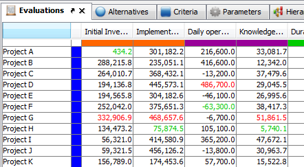
D-Sight is launched by default with the five main input panels. The first one is the Evaluations panel gathering all the alternatives (Project A, Project B …) and all the criteria. They are respectively represented in each row and each column. As shown in Figure 1 (click on the image to see the complete table), the evaluations can be numerical or based on qualitative scales.

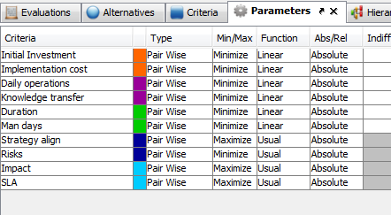
The two following panels allow the decision maker to list the alternatives and criteria. Names and short names can also be assigned to all these elements. The fourth panel introduces the evaluation parameters and is represented in Figure 2 below that allows the interested reader to consult the parameters used in this case.

 

 

 

 

 

 

 

 

 

 

 

 

 

 

 

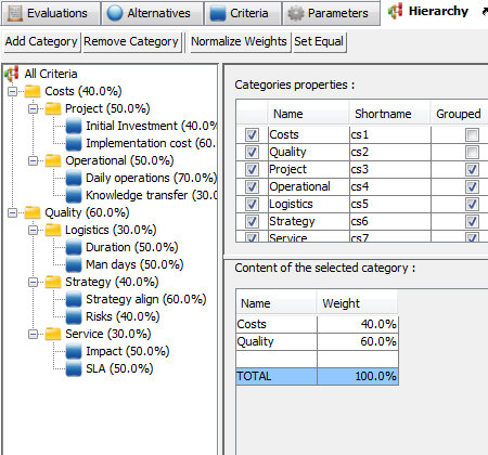
The last of the five panels allows structuring the criteria into a hierarchy tree. Categories can be defined in order to gather criteria or other categories or both. This tree can easily be constructed by dragging and dropping its elements.

The categories are defined in that panel. As represented in Figure 3, each category has a name, a short name and a color. They have two additional interesting properties:

The first one is that they can be disabled, just like the criteria or alternatives. The exception in this case is that when a category is enabled / disabled, all its content is automatically enabled / disabled. The last property of a category is that it can be grouped or ungrouped. This will be illustrated later on.

 

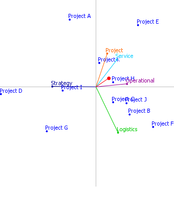
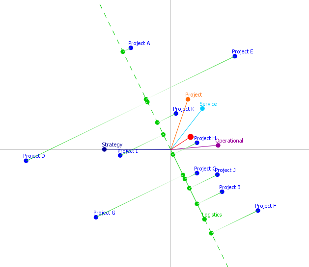
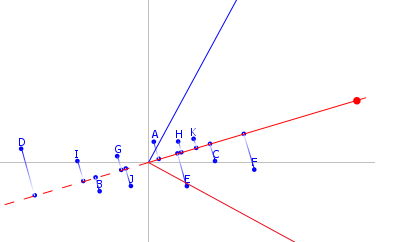
The Global Visual Analysis offers a complete overview of the problem. As shown in the figures below, the alternatives are represented by the blue points and the criteria are represented by the different axes. Please note that the criteria are not represented “as is” but according to the decision maker’s preferences (e.g. the preferences functions). The computation of this chart depends on two things:

• the alternatives and their gross criteria evaluations;
• the intra-criterion parameters expressing the way the decision maker wants to evaluate these alternatives for the different criteria.

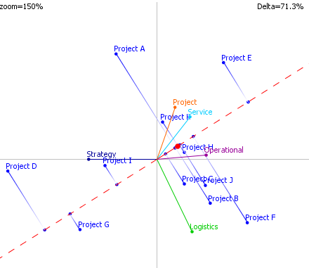
Since the decision maker has defined a hierarchy, he can choose what he wants to see in the GAIA plane by grouping or ungrouping the categories. In the three following figures, the Costs and Quality categories are ungrouped. Their respective subcategories are represented as they are ungrouped. Thanks to this plane and the “grouping” functionality, the alternatives can easily be compared on different levels of detail. Different points can now be observed:

 

Relative position of the alternatives: if two projects are close in the plane, as J and B, it means that they are be similar with respect to the different criteria.

Alternatives and criteria: an axis indicates the direction of the area in which the alternatives are good for the associated criterion. In the second figure below, the decision maker can observe that F is the best alternative for the global Logistics criterion (e.g. F’s projection is the highest on the Logistics axis).

Relative positions of the criteria: if two criteria axes point in the same direction, that indicates that they are similar (e.g. overall, the projects that score high for the first criterion, also score high for the second). If two criteria axes point in opposite directions, that means that they are conflicting (e.g. overall, the projects that score low for the first criterion also score low the second). In the following illustration, one can observe that on average, the projects having interesting Strategy scores are not good on the Operational aspects (i.e. the Strategy axis is situated on the left while the Operational axis is oriented to the right).

The red axis (the one without label) of the GAIA plane is called the decision axis. It is obtained by using the weights of the criteria given by the decision maker. It represents the compromise he wants to make between the criteria. By projecting the projects on this axis, the global ranking can be visualized as shown hereunder.

We would like to emphasize that the ranking deduced visually by projecting the alternatives on the criteria axes or on the decision axis may not be completely correct. This is due to the fact that a two-dimensional representation of a k-dimensional problem is used. For more information, please consult the complete PDF article.

 

 

 

 

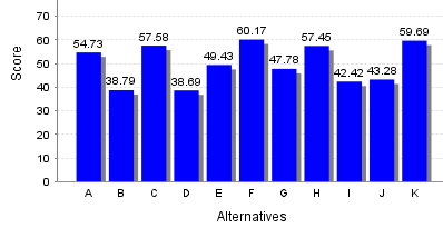
The PROMETHEE II ranking offers a total ranking of the alternatives from the best (the highest rank) to the worst (the lowest rank). They are scored between 0 and 100; 100 being the best. The ranking of the projects is represented in the illustration below. Project F ranks first with a score of 60.17, closely followed by project K, with a score of 59.69.

 

 

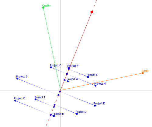
In the previous section, we mentioned that the visual global ranking can be obtained by projecting the alternatives on the decision axis. In the figure below, we have grouped the two main categories, Quality and Costs, which avoids loss of information (since this is a two dimensional representation).

The delta value is, in this case equal to 100%. One can now observe that the projections of the alternatives on the decision axis do perfectly reflect the PROMETHEE II ranking, with the ordinal and cardinal information.

 

 

Another interesting point related to this visual configuration, is that it allows quantifying the Quality / Cost trade-off that exists when choosing one project over another. Indeed, one can observe that choosing between F and K, that are almost equally scored in PROMETHEE II, is equivalent to choosing between Quality and Costs.

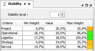
In most multi-criteria analyses, the assessment of criteria weights is a crucial step. Indeed, these weights have a large influence on the global score calculation. Therefore, it is important to perform sensitivity analyses. In D-Sight, this is done by using the stability intervals. They give, for each criterion or category (according to the decision maker’s choice), the interval in which the weights can vary without affecting the ranking.

 

We can observe in the figure opposite, that some of these values are rather robust while others are more instable. An important point to emphasize here is the following: one could think that the Logistics category is stable because the weight can increase from 18% to 100% without affecting the ranking (to the level 1). But on the other hand, it cannot even be decreased by 1% without affecting the ranking. That means that Logistics is only stable “on the right side”. This table shows us that there is some asymmetry in the stability. The following hypothesis is here considered: when a weight is changed, the other weights are proportionally changed, with respect to the initial ratios. The stability level is the rank to which the stability is considered. In the present case, the level is one which means that we only look at the first alternative and in which intervals it stays first, regardless if the third alternative becomes second. The stability level can be calculated up to n. The bigger the level is, the smaller the intervals are, as constraints are added.

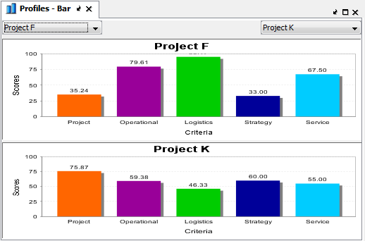
The previous analysis has led us to identify a sub group of alternatives that are more interesting than others. Clearly, F and K seem to be good candidates. A natural next step is thus to focus ourselves on the differentiation between these two options. The profiles of the alternatives can be compared two by two by using the Profiles tool. In the following figure, F and K are compared for all the level-2 categories. It is easy to see that they do not have similar profiles, especially for the Project, Logistics and the Strategy criteria.

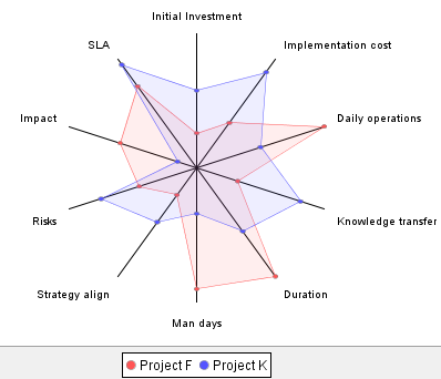
The same type of analysis can be made in a spider-web chart, as represented below. In this case, we compare the two first alternatives, F and K, for all the sub criteria (level 3). We have ungrouped all the categories, which automatically updates the chart.

Thanks to this chart, one can observe that K (K is the one that scores best on the Risks) has a more balanced good profile. On the other hand, F has strong points while it is very weak on others.

 

 

We will now consider the case in which the decision maker has to select several projects. He thus needs to establish the best project portfolio. Having ranked all the projects by attractiveness, the decision maker will have to determine which projects he will select in order to respect some imposed constraints.

This problem consists in selecting the best subset of alternatives (with respect to their global scores) while considering different constraints. To illustrate this, we will use the sub-set optimization plugin that is available for D-Sight. This plugin is based on the PROMETHEE V method.

The process is divided in two steps:

1. A ranking of the alternatives / projects is established, considering the preferences of the decision maker. The alternatives are ranked with respect to their attractiveness for the decision maker without taking any constraints or relation between the alternatives into account.
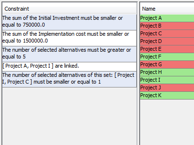
2. The decision maker can provide constraints such as a budget or a minimum number of alternatives to be selected, for instance. A subset of alternatives is then found to maximize the total additive score of the subset while respecting all the established constraints.

We will now come back to the example in order to illustrate the use of this plugin. Imagine that Production Inc. wants to implement different projects but needs to respect the following constraints:

• A limited Initial investment of 750.000 €.
• A limited Implementation Cost of 1.500.000€.
• The number of selected projects must be greater or equal to 5.
• If project A is selected, project I must be selected.
• If project I is selected, project C can’t be and vice-versa.

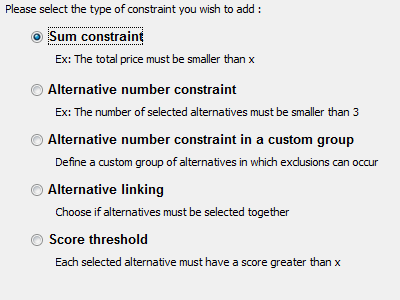
The different constraints can be defined into an interface as illustrated in the following figure.

 

 

 

 

As the constraints are being added, the subset is gradually computed taking into account the additional constraints. Finally, the optimal subset is calculated (that is, if a solutions exists). As illustrated below, the selected alternatives are highlighted in green in the table. The “Show Everywhere” button allows displaying the green (selected) and red (not selected) colors in all the charts and tables of the software. This can help to integrate the optimization results in the other tools in order to make an easy global analysis.

Please note that many types of constraints can be defined. Furthermore, custom groups can also be defined in order to use group related constraints.

In this section, we will consider the case in which two decision makers are involved in the projects selection. Consider two managers, John and Jane.

As defined in the model, each participant works with the same set of alternatives and criteria (structured in the same way).

The participants can differentiate their analysis on three main points:

• The evaluation of the alternatives for the criteria: this is relevant for criteria based on qualitative judgments given by different experts.
• The evaluation parameters: the actors can decide not to evaluate the criteria in the same manner. They can have different functions or different thresholds.
• The weights of the criteria: each stakeholder can weigh the criteria according to his own preferences.

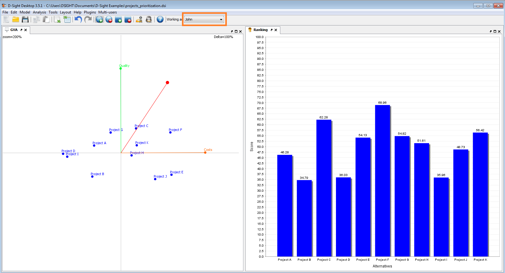
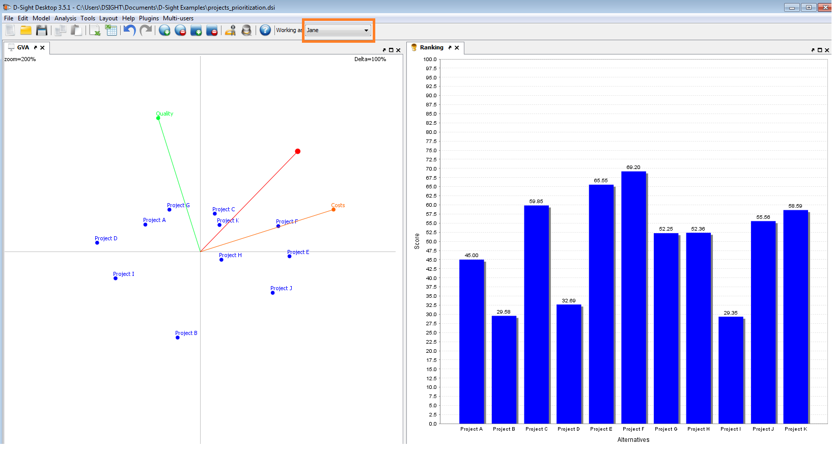
In the previous part of this article, John was the only decision maker in the selection process. We will consider that John and Jane will only weigh the criteria differently. Indeed, Jane accords more importance to the Costs than to the Quality. She has also given different weights to the sub-categories. In the left figure below, we have represented the visual analysis and the global ranking according to John’s preferences. We of course obtain the results previously presented.

 

 

 

 

To change the current decision-maker, one has to select the right user in the list. The entire interface is automatically updated with the corresponding data and results. In the right illustration above, Jane’s results are represented. The ranking of the alternatives is different and so is the GAIA plane. The reader could expect the GAIA plane to be the same in the two cases, except for the decision axis, as only the weights have changed. As the weights of the sub-categories are not the same for John and Jane, the unicriterion scores of the alternatives for the Quality and the Costs are different which explains the computation of two different planes.

As we have had a look at each stakeholder’s results, we can now analyze the global results. A new dedicated window is opened and organized the same way as the main one. It is represented in the following figure. Its look and feel can be set differently to be easily recognized by the user.

In the evaluation table, the projects are still represented in the rows but the columns do not represent the criteria anymore. Indeed, each column represents a decision maker. That means that this table contains the scores of the projects for the different stakeholders.

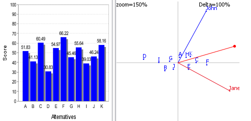
As each stakeholder is weighted, that allows computing a global aggregated score for all the projects. The following figure shows that project F is the preferred project while taking into account each stakeholder’s point of view. Furthermore, a GAIA plane can also be represented with the aggregated users. In this representation, the points are used for the projects but, as expected, the axes now represent the actors. The decision axis (the axis without label), is computed with respect to the weights given to the decision makers in order to represent the direction of the most globally preferred project.

If we take a closer look at the GAIA plane, we can see that there is a group of alternatives, situated in the left part that will never be chosen if both decision makers have to agree on the solution.

In the right part of the plane, two different subsets of projects are observable (represented below in more details with the projections):

• The conflicting projects (K, C, H): those solutions are well scored but are not preferred the same way by each stakeholders. For instance, project K is very good according to John but is only fourth according to Jane. In general, conflicting alternatives have crossing lines when projecting on the decision makers’ axes.
• The best consensus projects (project F): those solutions are preferred by all the decision makers. They have no crossing lines when projecting on the decision makers’ axis.

Figure 16 - Click to enlarge

 

 

The multi-actors plugin is now extended to an online group decision support system. This allows the stakeholders to work remotely as well as having different roles (e.g. project manager, expert …) in the decision process.